Chaining effect in clustering
Posted on Mon 21 January 2019 in machine learning • 5 min read
This post is part 5 of the "clustering" series:
- Generate datasets to understand some clustering algorithms behavior
- K-means is not all about sunshines and rainbows
- Gaussian mixture models: k-means on steroids
- How many red Christmas baubles on the tree?
- Chaining effect in clustering
- Animate intermediate results of your algorithm
- Accuracy: from classification to clustering evaluation
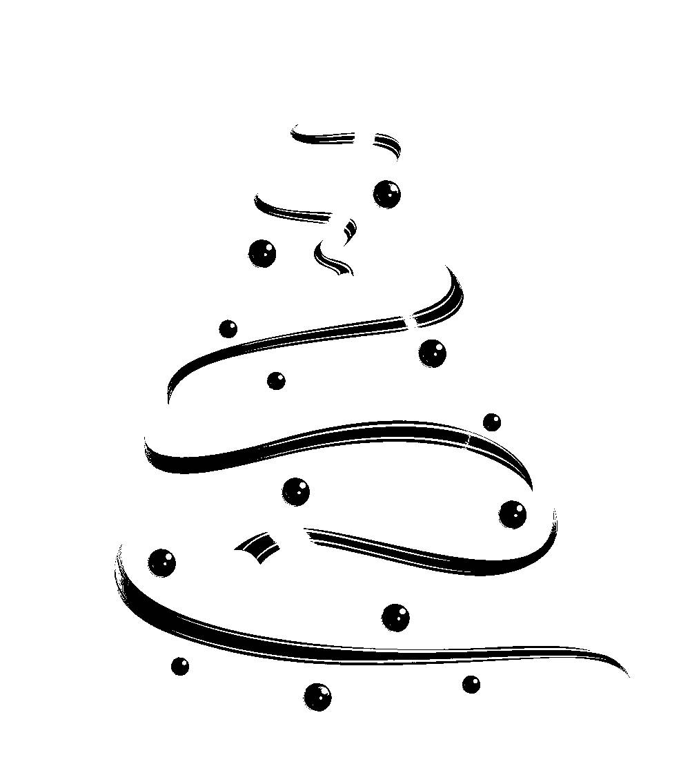
In a previous blog post, I explained how we can leverage the k-means clustering algorithm to count the number of red baubles on a Christmas tree. This method fails however if we put Christmas tinsels on it. Let’s find a solution for this more difficult case.

Filter red points
Let's first proceed as we did for Christmas baubles by filtering the red points from the others (download the image here):
library("jpeg")

filename = "tree.jpg"
a = readJPEG(filename)

library("dplyr")

getLayer <- function(a, n) {
    layer = a[, , n]
    layer = as.data.frame(as.table(layer))
    colnames(layer) <- c("x", "y", paste0("layer", n))
    layer
}

layer1 = getLayer(a, 1)
layer2 = getLayer(a, 2) %>% select(layer2)
layer3 = getLayer(a, 3) %>% select(layer3)
df = layer1 %>% bind_cols(layer2, layer3)

df = df %>% mutate(tmp = case_when(
    (layer1 > 0.5) & (layer1 > 2* layer2) ~ 0,
    TRUE ~ 1
)) %>% transmute(x=x, y=y, layer1=tmp, layer2=tmp, layer3=tmp)

library("abind")
library("tidyr")

createMatrixLayer <- function(df, n) {
    layerName = paste0("layer", n)
    d = df %>% select(x, y, layerName)
    d = spread(d, y, layerName) %>% select(-x)
    d
}

layer1 = createMatrixLayer(df, 1)
layer2 = createMatrixLayer(df, 2)
layer3 = createMatrixLayer(df, 3)

b = abind(layer1, layer2, layer3, along = 3)

writeJPEG(b, "red.jpg")
We filtered the points both from the red Christmas baubles and the tinsels:
Let's now see how we can create meaningful clusters.
Choose an algorithm
In order to cluster these points so that a cluster corresponds either to a red Christmas bauble or a Christmas tinsel, we have to find clusters which do not fit the k-means nor the Gaussian mixture models assumptions: the Christmas tinsels correspond to elongated classes.
The chaining effect of the hierarchical clustering with single linkage aggregation criterion fits perfectly this case: For a given set of points S in a Christmas tinsel, the most probable point to consider for inclusion into the same cluster, is the point which is the closest of any point of S.
The hierarchical clustering with single linkage works as follows:
- Put each point into its own cluster (for this step, the number of clusters is the same as the number of points).
- Create a proximity matrix where the proximity between two clusters A and B is calculated by: \(d(A, B) = \min_{x \in A, y \in B} || x - y ||\)
- Find the most similar pair of clusters according to the proximity matrix and join them together.
- Update the proximity matrix (there is one cluster less and we have to compute the proximities between the cluster created in the previous step and the others).
- Repeat steps 3 and 4 until all points are in the same cluster.
Reduce the input size
It happens that the hierarchical clustering is heavy since we have to compute the distances between all the points in the first step. We can first reduce the dimensionality of the input by a previous clustering step, with a lighter clustering algorithm: k-means has a complexity of \(k * n\) where \(k\) is the number of clusters and \(n\) is the number of points, whereas hierarchical clustering has a complexity of \(n^2\) for the first step.
We can group the points with k-means into a large enough number of clusters so that the points of the same Christmas bauble or tinsel are not spread across several clusters, while the dimensionality is reduced.
Let's apply k-means with 500 clusters and plot the centroids:
library("ggplot2")

df = df %>%
    filter(layer1==0) %>%
    mutate(tmp=as.numeric(y),
           y=-as.numeric(x),
           x=tmp) %>%
    select(x, y)

km = kmeans(df, 500, iter.max = 20, nstart = 10)

g = as.data.frame(km$centers) %>%
    ggplot(aes(x, y)) + geom_point()
g
Reducing the points to the centroids found by k-means keeps the shape of our data:

Apply hierarchical clustering with single linkage
We first cluster the points with k-means and then cluster the centroids of the clusters found by k-means to get our final clustering:
centers = as.data.frame(km$centers)
d = dist(centers, method="euclidean")
hc <- hclust(d, method = "single")
One advantage of hierarchical clustering is that we can set the number of clusters after the execution of the algorithm. The distances between the clusters at each level of the hierarchy help us select a good candidate for the number of clusters to choose. Let's see how the distances between the clusters evolve:
g = data_frame(y = hc$height) %>%
    arrange(desc(y)) %>%
    mutate(x=row_number()) %>%
    ggplot(aes(x, y)) +
    geom_point()
g
Here, we plotted the height attribute on the y axis, and the number of aggregations (\(k - 1\) where \(k\) is the number of clusters) on the x axis:

The height attribute is computed as follows: Let \(v\) denote the point such that:
where A and B are two clusters to merge. \(v\) is equidistant from all the points in A and B and \(delta\) defines an ultra-metric. \(h\) is the height for the iteration. The height attribute contains all the values of h (one value per iteration).
We can see drops between two consecutive points, which means that the clusters between two steps are far away when we observe the drop. Let's zoom on the area where we see the drops:
g = data_frame(y = hc$height) %>%
    arrange(desc(y)) %>%
    mutate(x=row_number()) %>%
    filter(x<=50) %>%
    ggplot(aes(x, y)) +
    geom_point()
g

When the number of clusters is more than 24, there is no drop: If we divide in more than 24 clusters, the clusters generated by the division are not well separated. 24 clusters is therefore a good candidate for the number of clusters since merging two clusters from the partition in 24 clusters result in a merge of two well separated clusters.
We can plot the dendrogram where we can see the hierarchy and the distances between each pair of clusters at each level of the hierarchy:
library(factoextra)

g = fviz_dend(hc, k=24, show_labels = FALSE)
g

Let's see the result of the clustering with 24 clusters:
library(ggrepel)

cluster <- cutree(hc, k = 24)

c = centers %>% bind_cols(as.data.frame(cluster)) %>%
    group_by(cluster) %>%
    summarise(x=first(x), y=first(y))


g = centers %>% bind_cols(as.data.frame(cluster)) %>%
    ggplot(aes(x, y, color=as.factor(cluster))) +
    geom_point() +
    geom_label_repel(data=c, aes(x, y, label=cluster), box.padding = 1) +
    theme(legend.position="none")

g

Take away
Here are a few things to remember from this blog post:
- Hierarchical clustering is handy since one can select the number of clusters a posteriori. A dendrogram provides a nice visualisation of the clustering steps and gives visual insights into how to choose a good number of clusters.
- K-means is a good pre-processing since it has a low time complexity. We can then apply another clustering algorithm on the centroids found by k-means.
- The single linkage aggregation criterion for hierarchical clustering is well suited when we seek elongated clusters because of its chaining effect.